In Part I, we saw a few examples of image classification. In particular counting objects seemed to be difficult for convolutional neural networks. After sharing my work on the fast.ai forums, I received a few suggestions and requests for further investigation.
The most common were:
Some transforms seemed uneccessary (eg. crop and zoom)
Some transforms might be more useful (eg. vertical flip)
Consider training the model from scratch (inputs come from a different distribution)
Try with more data
Try with different sizes
Sensible Transforms
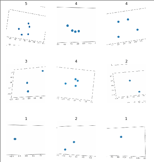
After regenerating our data we can look at it:
Looks better, all transforms keep the dots centered and identical
Now we can create a learner and train it on this new dataset.
This file contains bidirectional Unicode text that may be interpreted or compiled differently than what appears below. To review, open the file in an editor that reveals hidden Unicode characters. Learn more about bidirectional Unicode characters
Wow! Look at that, this time we’re getting 100% accuracy. It looks like if we throw enough data at it (and use proper transforms) this is a problem that can actually be trivially solved by convolutional neural networks. I honestly did not expect that at all going into this.
Different Sizes of Objects
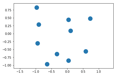
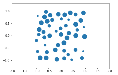
One drawback of our previous dataset is that the objects we’re counting are all the same size. Is it possible this is making the task too easy? Let’s try creating a dataset with circles of various sizes.
This file contains bidirectional Unicode text that may be interpreted or compiled differently than what appears below. To review, open the file in an editor that reveals hidden Unicode characters. Learn more about bidirectional Unicode characters
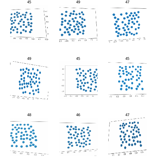
Which allows us to create images that look something like:
Objects of various sizes
Once again we can create a dataset this way and train a convolutional learner on it. Complete code on GitHub.
Results:
1
1.075099
0.807987
0.381000
2
0.613711
5.742334
0.796600
…
…
…
…
14
0.009446
0.000067
0.000000
15
0.001920
0.000075
0.000000
Still works! Once again I’m surprised. I had very little hope for this problem but these networks seem to have absolutely no issue with solving this.
This runs completely contrary to my expectations. I didn’t think we could count objects by classifying images. I should note that the network isn’t “counting” anything here, it’s simply putting each image into the class it thinks it would belong to. For example, if we showed it an example with 10 images, it would have to classify it as either “45”, “46”, “47”, “48” or “49”.
More generally, counting would probably make more sense as a regression problem than a classification problem. Still, this could be useful when trying to distinguish between object counts of a fixed and guaranteed range.
Over the last year I focused on what some call a “bottom-up” approach to studying deep learning. I reviewed linear algebra and calculus. I read Ian Goodfellow’s book “Deep Learning”. I built AlexNet, VGG and Inception architectures with TensorFlow.
While this approach helped me learn the bits and bytes of deep learning, I often felt too caught up in the details to create anything useful. For example, when reproducing a paper on superconvergence, I built my own ResNet from scratch. Instead of spending time running useful experiments, I found myself debugging my implementation and constantly unsure if I’d made some small mistake. It now looks like I did make some sort of implementation error as the paper was successfully reproduced by fast.ai and integrated into fast.ai’s framework for deep learning.
With all of this weighing on my mind I found it interesting that fast.ai advertised a “top-down” approach to deep learning. Instead of starting with the nuts and bolts of deep learning, they instead first seek to answer the question “How can you make the best/most accurate deep learning system?” and structure their course around this question.
The first lesson focuses on image classification via transfer learning. They provide a pre-trained ResNet-34 network that has learned weights using the ImageNet dataset. This has allowed it to learn various things about the natural world such as the existence of edges, corners, patterns and text.
After creating a competent pet classifier they recommend that students go out and try to use the same approach on a dataset of their own creation. For my part I’ve decided to try their approach on three different datasets, each chosen to be slightly more challenging than the last:
Our first step is simply to import everything that we’ll need from the fastai library:
This file contains bidirectional Unicode text that may be interpreted or compiled differently than what appears below. To review, open the file in an editor that reveals hidden Unicode characters. Learn more about bidirectional Unicode characters
Next we’ll take a look at the data itself. I’ve saved it in data/paintings. We’ll create an ImageDataBunch which automatically knows how to read labels for our data based off the folder structure. It also automatically creates a validation set for us.
This file contains bidirectional Unicode text that may be interpreted or compiled differently than what appears below. To review, open the file in an editor that reveals hidden Unicode characters. Learn more about bidirectional Unicode characters
Looking at the above images, it’s fairly easy to differentiate the solid lines of modernism from the soft edges and brush strokes of impressionist paintings. My hope is that this task will be just as easy for a pre-trained neural network that can already recognize edges and identify repeated patterns.
Now that we’ve prepped our dataset, we’ll prepare a learner and let it train for five epochs to get a sense of how well it does.
This file contains bidirectional Unicode text that may be interpreted or compiled differently than what appears below. To review, open the file in an editor that reveals hidden Unicode characters. Learn more about bidirectional Unicode characters
Looking good! With virtually no effort at all we have a classifier that reaches 95% accuracy. This task proved to be just as easy as expected. In the notebook we take things a further by choosing better learning rate and training for a little while longer before ultimately getting 100% accuracy.
The painting task ended up being as easy as we expected. For our second challenge we’re going to look at a dataset of about 180 cats and 180 kittens. Cats and kittens share many features (fur, whiskers, ears etc.) which seems like it would make this task harder. That said, a human can look at pictures of cats and kittens and easily differentiate between them.
This time our data is located in data/kittencat so we’ll go ahead and load it up.
This file contains bidirectional Unicode text that may be interpreted or compiled differently than what appears below. To review, open the file in an editor that reveals hidden Unicode characters. Learn more about bidirectional Unicode characters
Once again, let’s try a standard fastai CNN learner and run it for about 5 epochs to get a sense for how it’s doing.
This file contains bidirectional Unicode text that may be interpreted or compiled differently than what appears below. To review, open the file in an editor that reveals hidden Unicode characters. Learn more about bidirectional Unicode characters
So we’re looking at about 86% accuracy. Not quite the 95% we saw when classifying paintings but perhaps we can push it a little higher by choosing a good learning rate and running our model for longer.
Below we are going to use the “Learning Rate Finder” to (surprise, surprise) find a good learning rate. We’re looking for portions of the plot in which the graph steadily decreased.
This file contains bidirectional Unicode text that may be interpreted or compiled differently than what appears below. To review, open the file in an editor that reveals hidden Unicode characters. Learn more about bidirectional Unicode characters
It looks like there is a sweetspot between 1e-5 and 1e-3. We’ll shoot for the ‘middle’ and just use 1e-4. We’ll also run for 15 epochs this time to allow more time for learning.
This file contains bidirectional Unicode text that may be interpreted or compiled differently than what appears below. To review, open the file in an editor that reveals hidden Unicode characters. Learn more about bidirectional Unicode characters
Not bad! With a little bit of learning rate tuning, we were able to get a validation accuracy of about 92% which is much better than I expected considering we had less than 200 examples of each class. I imagine if we collected a larger dataset we could do even better.
For my last task I wanted to see whether or not we could train a ResNet to “count” identical objects. So far we have seen that these networks excel at distinguishing between different objects, but can these networks also identify multiple occurrences of something?
Note: I specifically chose this task because I don’t believe it should be possible for a vanilla ResNet to accomplish this task. A typical convolutional network is set up to differentiate between classes based on the features of those classes, but there is nothing in a convolutional network that suggests to me that it should be able to count objects with identical features.
For this challenge we are going to synthesize our own dataset using matplotlib. We’ll simply generate plots with the correct number of circles in them as shown below:
This file contains bidirectional Unicode text that may be interpreted or compiled differently than what appears below. To review, open the file in an editor that reveals hidden Unicode characters. Learn more about bidirectional Unicode characters
When we create a dataset like this, we’re in uncharted territory as far as the pre-trained weights are concerned. Our network was trained on photographs of the natural world and expects its inputs to come from this distribution. We’re providing inputs from a completely different distribution (not necessarily a harder one!) so I wouldn’t expect transfer learning to work as flawlessly as it did in previous examples.
Our dataset might be trivially easy to learn. For example, if we wrote an algorithm that simply counted the number of “blue” pixels we could very accurately figure out how many circles were present as all circles are the same size.
We don’t need to hypothesize any further, though. We can just create our ImageDataBunch and pass it to a learner to see how well it does. For now we’ll just use a dataset with 1-5 elements.
This file contains bidirectional Unicode text that may be interpreted or compiled differently than what appears below. To review, open the file in an editor that reveals hidden Unicode characters. Learn more about bidirectional Unicode characters
Samples from our dataset. Notice how fastai automatically performs data augmentation for us!
Let’s create our learner and see how well it does with the defaults after 3 epochs.
This file contains bidirectional Unicode text that may be interpreted or compiled differently than what appears below. To review, open the file in an editor that reveals hidden Unicode characters. Learn more about bidirectional Unicode characters
So without any changes we’re sitting at over 85% accuracy. This surprised me as I thought this task would be harder for our neural network as each object it was counting has identical features. If we run this experiment again with a learning rate of 1e-4 and for 15 cycles things get even better:
epoch
train_loss
valid_loss
error_rate
1
0.657094
0.406908
0.133000
2
0.632255
0.337327
0.100000
…
…
…
…
14
0.236516
0.039613
0.002000
15
0.264761
0.037968
0.002000
Wow! We’ve pushed the accuracy up to 99%!
Ugh. This seems wrong to me…
I am not a deep learning pro but every fiber of my being screams out against convolutional networks being THIS GOOD at this task. I specifically chose this task to try to find a failure case! My understanding is that they should be able to identify composite features that occur in an image but there is nothing in there that says they should be able to count (or have any notion of what counting means!)
What I would guess is happening here is that there are certain visual patterns that can only occur for a given number of circles (for example, one circle can never create a line) and that our network uses these features to uniquely identify each class. I’m not sure how to prove this but I have an idea of how we might break it. Maybe we can put so many circles on the screen that the unique patterns will become very hard to find. For example, instead of trying 1-5 circles, let’s try counting images that have 45-50 circles.
After re-generating our data (see Notebook for details) we can visualize it below:
This file contains bidirectional Unicode text that may be interpreted or compiled differently than what appears below. To review, open the file in an editor that reveals hidden Unicode characters. Learn more about bidirectional Unicode characters
Now we can run our learner against this and see how it does:
This file contains bidirectional Unicode text that may be interpreted or compiled differently than what appears below. To review, open the file in an editor that reveals hidden Unicode characters. Learn more about bidirectional Unicode characters
Hah! That’s more like it. Now our network can only achieve ~25% accuracy which is slightly better than chance (1 in 5). Playing around with learning rate I was only able to achieve 27% on this task.
This makes more sense to me. There are no “features” in this image that would allow a network to look at it and instantly know how many circles are present. I suspect most humans can also not glance at one of these images and know whether or not there are 45 or 46 elements present. I suspect we would have to fall back to a different approach and manually count them out.
Update
It turns out that we CAN make this work! We just have to use more sensible transformations. For more info see my next post: Image Classification: Counting Part II.
At the end of last year’s retrospective, I set a number of goals for myself. It feels (really) bad to look back and realize that I did complete a single one. I think it’s important to reflect on failures and shortcomings in order to understand them and hopefully overcome them going forward.
Goal 1: Write one blog post every week
Result: 13 posts / 52 weeks
In January 2018 I began the blog series Learn TensorFlow Now which walked users through the very basics of TensorFlow. For three months I stuck to my goal of writing one blog post every week and I’m very proud of how my published posts turned out. Unfortunately during April I took on a consulting project and my posts completely halted. Once I missed a single week I basically gave up on blogging altogether. While I don’t regret taking on a consulting project, I do regret that I used it as an excuse to stop blogging.
This year I would like to start over and try once again to write one blog post per week (off to a rough start considering it’s already the end of January!). I don’t really have a new strategy other than I will resolve not to quit entirely if I miss a week.
When I first started reading this book I was very intimidated by the first few chapters covering the background mathematics of deep learning. While my linear algebra was solid, my calculus was very weak. I put the book away for three months and grinded through Khan Academy’s calculus modules. I say “grinded” because I didn’t enjoy this process at all. Every day felt like a slog and my progress felt painfully slow. Even knowing calculus would ultimately be applicable to deep learning, I struggled to stay focused and interested in the work.
When I came back to the book in the second half of 2018 I realized it was a mistake to stop reading. While the review chapters were mathematically challenging, the actual deep learning portions were much less difficult and most of the insights could be reached without worrying about the math at all. For example, I cannot prove to you that L1 regularization results in sparse weight matrices, but I am aware that such a proof exists (at least in the case of linear regression).
This year I would like to finish this book. I think it might be worth my time to try to implement some of the basic algorithms illustrated in the book without the use of PyTorch or TensorFlow, but that will remain a stretch goal.
Goal 3: Contribute to TensorFlow
Result: 1 Contribution?
In February one of my revised PRs ended up making it into TensorFlow. Since I opened it in December of the previous year I’ve only marked it as half a contribution. Other than this PR I didn’t actively seek out any other places where I could contribute to TensorFlow.
On the plus side, I recently submitted a pull request to PyTorch. It’s a small PR that helps bring the C++ API closer to the Python API. Since it’s not yet merged I guess I should only count this as half a contribution? At least that puts me at one full contribution to deep learning libraries for the year.
Goal 4: Compete in a more Challenging Kaggle competition
Result: 0 attempts
There’s not much to say here other than that I didn’t really seek out or attempt any Kaggle competitions. In the later half of 2018 I began to focus on reinforcement learning so I was interested in other competitive environments such as OpenAI Gym and Halite.io. Unfortunately my RL agents were not very competitive when it came to Halite, but I’m hoping this year I will improve my RL knowledge and be able to submit some results to other competitions.
Goal 5: Work on HackerRank problems to strengthen my interview skills
Result: 3 months / 12 months
While I started off strong and completed lots of problems, I tapered off around the same time I stopped blogging. While I don’t feel super bad about stopping these exercises (I had started working, after all) I am a little sad because it didn’t really feel like I improved at solving questions. This remains an area I want to improve in but I don’t think I’m going to make it an explicit goal in 2019.
Goal 6: Get a job related to ML/AI
Result: 0 jobs
I did not receive (or apply to) any jobs in ML/AI during 2018. After focusing on consulting for most of the year I didn’t feel like I could demonstrate that I was proficient enough to be hired into the field. My understanding is that an end-to-end personal project is probably the best way to demonstrate true proficiency and something I want to pursue during 2019.
Goals for 2019
While I’m obviously not thrilled with my progress in 2018 I try not to consider failure a terminal state. I’m going to regroup and try to be more disciplined and consistent when it comes to my work this year. One activity that I’ve found both fun and productive is streaming on Twitch. I spent about 100 hours streaming and had a pretty consistent schedule during November and December.
In the last few posts we noticed a strange phenomenon: our test accuracy was about 10% worse than what we were getting on our training set. Let’s review the results from our last network:
Cost: 131.964
Accuracy: 11.9999997318 %
...
Cost: 0.47334
Accuracy: 83.9999973774 %
Test Cost: 1.04789093912
Test accuracy: 72.5600001812 %
Our neural network is getting ~84% accuracy on the training set but only ~73% on the test set. What’s going on and how do we fix it?
Bias and Variance
Two primary sources of error in any machine learning algorithm come from either underfitting or overfitting your training data. Underfitting occurs when an algorithm is unable to model the underlying trend of the data. Overfitting occurs when the algorithm essentially memorizes the training set but is unable to generalize and performs poorly on the test set.
Bias is error introduced by underfitting a dataset. It is characterized by poor performance on both the training set and the test set.
Variance is error introduced by overfitting a dataset. It is characterized by a good performance on the training set, but a poor performance on test set.
We can look at bias and variance visually by comparing the performance of our network on the training set and test set. Recall our training accuracy of 84% and test accuracy of 73%:
Visualization of bias and variance from our previous network’s results
The above image roughly demonstrates which portions of our error can be attributed to bias and variance. This visualization assumes that we could theoretically achieve 100% accuracy. In practice this may not always be the case as other sources of error (eg. noise or mislabelled examples) may creep into our dataset. As an aside, the lowest theoretical error rate on a given problem is called the Bayes Error Rate.
Reducing Error
Ideally we would have a high performance on both the test set and training set which would represent low bias and low variance. So what steps can we take to reduce each of these sources of error?
Reducing Bias
Create a larger neural network. Recall that high bias is a sign that our neural network is unable to properly capture the underlying trend in our dataset. In general the deeper a network, the more complex the functions it can represent.
Train it for a very long time. One sanity check for any neural network is to see whether or not it can memorize the dataset. A sufficiently deep neural network should be able to memorize your dataset given enough training time. Although this won’t fix any problems with variance it can be an assurance that your network isn’t completely broken in some way.
Use a different architecture. Sometimes your chosen architecture may simply be unable to perform well on a given task. It may be worth considering other architectures to see if they perform better. A good place to start with Image Recognition tasks is to try different architectures submitted to previous ImageNet competitions.
Reducing Variance
Get more data. One nice property of neural networks is that they typically generalize better and better as you feed them more data. If your model is having problems handling out-of-sample data one obvious solution is to feed it more data.
Augment your existing data. While “Get more data” is a simple solution, it’s often not easy in practice. It can take months to curate, clean and verify a large dataset. One workaround is to artifically generate “new” data by augmenting your existing data. For image recognition tasks this might include flipping or rotating existing images, tweaking color settings or taking random crops of images. This is a topic we’ll explore in greater depth in future posts.
Regularization. High variance with low bias suggests our network has memorized the training set. Regularization describes a class of modifications we can make to our neural network that either penalizes memorization (eg. L2 regularization) or promotes redundant paths of learning in our network (ie. Dropout). We will dive deeper into various regularization approaches in future posts.
Use a different architecture. Like reducing bias, sometimes you get the most bang-for-your-buck when you switch architectures altogether. As the deep learning field grows, people are frequently discovering better architectures for certain tasks. Some recent papers have even suggested that the structure of a neural network is more important than any learned weights for that structure.
There’s a lot to unpack here and we’ve glossed over many of the solutions to the problems of bias and variance. In the next few posts we’re going to revisit some of these ideas and explore different areas of the TensorFlow API that allow us to tackle these problems.
In previous posts, we simply passed raw images to our neural network. Other forms of machine learning pre-process input in various ways, so it seems reasonable to look at these approaches and see if they would work when applied to a neural network for image recognition.
Zero Centered Mean
One characteristic we desire from any learning algorithm is for it to generalize across different input distributions. For example, let’s imagine we design an algorithm for predicting whether or not the price of a house is “High” or “Low“. As input it takes:
Number of Rooms
Price of House
Below is some made-up data for the city of Boston. I’ve marked “High” in red, “Low” in blue and a reasonable decision boundary that our algorithm might learn in black. Our decision boundary correctly classifies all examples of “High” and “Low“.
Classification of house prices in Boston
What happens when we take this model and apply it to houses in New York where houses are much more expensive? Below we can see that the model does not generalize and incorrectly classifies many “Low” house prices as “High“.
Classification of house prices in New York
In order to fix this, we want to take all of our data and zero-center it. To do this, we subtract the mean of each feature from from each data-point. For our examples this would look something like:
Zero centering the mean for Boston housing dataZero centering the mean for New York housing data
Notice that we zero-center the mean for both the “Price” feature as well as the “Number of Rooms” feature. In general we don’t know which features might cause problems and which ones will not, so it’s easier just to zero-center them all.
Now that our data has a zero-centered mean, we can see how it would be easier to draw a single decision boundary that would accurately classify points from both Boston and New York. Zero centering our mean is one technique for handling data that comes from different distributions.
Changing Distributions in Images
It’s easy to see how the distribution of housing prices changes in different cities, but what would changes in distribution look like when we’re talking about images? Let’s imagine that we’re building an image classifier to distinguish between pictures of cats and pictures of dogs. Below is some sample data:
Training Data
Training images for our Cat vs. Dog classifier
Test Data
Test data for our Cat vs. Dog classifier
In the above classification task our cat images are coming from different distributions in our training and test sets. Our training set seems to contain exclusively black cats while our test set has a mix of colors. We would expect our classifier to fail on this task unless we take some time to fix our distribution problems. One way to fix this problem would be to fix our training set and ensure it contains many different colors of cats. Another approach we might take would be to zero-center the images, as we did with our housing prices.
Zero Centering Images
Now that we understand zero-centered means, how can we use this to improve our neural network? Recall that each pixel in an image is a feature, analogous to “Price” or “Number of Rooms” in our housing example. Therefore, we have to calculate the mean value for each pixel across the entire dataset. This gives us a 32x32x3 “mean image” which we can then subtract from every image we pass to our neural network.
You mean have noticed that the mean_image was automatically created for us when we called cifar_data_loader.load_data():
This file contains bidirectional Unicode text that may be interpreted or compiled differently than what appears below. To review, open the file in an editor that reveals hidden Unicode characters. Learn more about bidirectional Unicode characters
The mean image for the CIFAR-10 dataset looks something like:
Mean Image for CIFAR-10 dataset
Now we simply need to subtract the mean image from the input images in our neural network:
This file contains bidirectional Unicode text that may be interpreted or compiled differently than what appears below. To review, open the file in an editor that reveals hidden Unicode characters. Learn more about bidirectional Unicode characters
A test accuracy of 72.5% is a marginal increase over our previous result of 70.9% and it’s possible that our improvement is entirely due to chance. So why doesn’t zero centering the mean help much? Recall that zero-centering the mean leads to the biggest improvements when our data comes from different distributions. In the case of CIFAR-10, we have little reason to suspect that our portions of our images are obviously of different distributions.
Despite seeing only marginal improvements, we’ll continue to subtract the mean image from our input images. It imposes only a very small performance penalty and safeguards us against problems with distributions we might not anticipate in future datasets.
Over the last nine posts, we built a reasonably effective digit classifier. Now we’re ready to enter the big leagues and try out our VGGNet on a more challenging image recognition task. CIFAR-10 (Canadian Institute For Advanced Research) is a collection of 60,000 cropped images of planes, cars, birds, cats, deer, dogs, frogs, horses, ships, and trucks.
50,000 images in the training set
10,000 images in the test set
Size: 32×32 (1024 pixels)
3 Channels (RGB)
10 output classes
Sample images from CIFAR-10
CIFAR-10 is a natural next-step due to its similarities to the MNIST dataset. For starters, we have the same number of training images, testing images and output classes. CIFAR-10’s images are of size 32x32 which is convenient as we were paddding MNIST’s images to achieve the same size. These similarities make it easy to use our previous VGGNet architecture to classify these images.
Despite the similarities, there are some differences that make CIFAR-10 a more challenging image recognition problem. For starters, our images are RGB and therefore have 3 channels. Detecting lines might not be so easy when they can be drawn in any color. Another challenge is that our images are now 2-D depictions of 3-D objects. In the above image, the center two images represent the “truck” class, but are shown at different angles. This means our network has to learn enough about “trucks” to recognize them at angles it has never seen before.
In order to make it easier to work with, I’ve prepared a small script that downloads, shuffles and caches the dataset locally. You can find it on GitHub here.
After saving this file locally, we can use it to prepare our datasets:
This file contains bidirectional Unicode text that may be interpreted or compiled differently than what appears below. To review, open the file in an editor that reveals hidden Unicode characters. Learn more about bidirectional Unicode characters
The above output shows that we’ve downloaded the dataset and created a training set of size 50,000 and a test set of size 10,000. Note: Unlike MNIST, these labels are not 1-hot encoded (otherwise they’d be of size 50,000x10 and 10,000x10 respectively). We have to account for this difference in shape when we build VGGNet for this dataset.
Let’s start by adjusting input and labels to fit the CIFAR-10 dataset:
This file contains bidirectional Unicode text that may be interpreted or compiled differently than what appears below. To review, open the file in an editor that reveals hidden Unicode characters. Learn more about bidirectional Unicode characters
Next we have to adjust the first layer of our network. Recall from the post on convolutions that each convolutional filter must match the depth of the layer against which it is convolved. Previously we had defined our convolutional filter to be of shape [3, 3, 1, 64]. That is, a 643x3 convolutional filters, each with depth of 1, matching the depth of our grayscale input image. Now that we’re using RGB images, we must define it to be of shape [3, 3, 3, 64]:
This file contains bidirectional Unicode text that may be interpreted or compiled differently than what appears below. To review, open the file in an editor that reveals hidden Unicode characters. Learn more about bidirectional Unicode characters
Another change we must make is the calculation of cost. Previously we were using tf.nn.softmax_cross_entropy_with_logits() which is suitable only when our labels are 1-hot encoded. When we represent the labels as single integers, we can instead use tf.nn.sparse_softmax_cross_entropy_with_logits(). It is otherwise identical to our original softmax cross entropy function.
This file contains bidirectional Unicode text that may be interpreted or compiled differently than what appears below. To review, open the file in an editor that reveals hidden Unicode characters. Learn more about bidirectional Unicode characters
Finally, we must also modify our calculation of correction_prediction (used to calculate accuracy) to account for the change in label shape. We no longer have to take the tf.argmax of our labels because they’re already represented as a single number:
This file contains bidirectional Unicode text that may be interpreted or compiled differently than what appears below. To review, open the file in an editor that reveals hidden Unicode characters. Learn more about bidirectional Unicode characters
Our final test accuracy appears to be approximately 71%, which isn’t too great. On one hand this is disappointing as it means our VGGNet architecture (or the method in which we’re training it) doesn’t generalize very well. On the other hand, CIFAR-10 presents us with new opportunities to try out new neural network components and architectures. In the next few posts we’ll explore some of these approaches to build a neural network that can handle the more complex CIFAR-10 dataset.
If you look carefully at the previous results you may have noticed something interesting. For the first time, our test accuracy (71%) is much lower than our training accuracy (~82-87%). This is a problem we’ll discuss in future posts on bias and variance in deep learning.
Complete Code
This file contains bidirectional Unicode text that may be interpreted or compiled differently than what appears below. To review, open the file in an editor that reveals hidden Unicode characters. Learn more about bidirectional Unicode characters
In the last post we looked at a modified version of VGGNet that achieved ~97.8% accuracy recognizing handwritten digits. Now that we’re relatively satisfied with our network, we’d like to save a trained version of the network that we can restore and use to classify digits whenever we’d like. We’ll do so by saving all of the tf.Variables() we’ve created to a checkpoint (.ckpt) file.
Saving a Checkpoint
When we save our computational graph, we serialize both the graph itself and the values of all of our parameters. When serializing nodes in our graph, TensorFlow keeps track of their names in order for us to interact with them later. Nodes that we don’t name will receive default names and be very hard to pick out. (While preparing this post I forgot to name input and labels which received the names Placeholder and Placeholder_1 instead). For this reason, we’ll take a minute to ensure that we give names to input, labels, cost, accuracy and predictions.
This file contains bidirectional Unicode text that may be interpreted or compiled differently than what appears below. To review, open the file in an editor that reveals hidden Unicode characters. Learn more about bidirectional Unicode characters
Saving a single checkpoint is straightforward. If we just want to save the state of our network after training then we simply add the following lines to the end of our previous network:
This file contains bidirectional Unicode text that may be interpreted or compiled differently than what appears below. To review, open the file in an editor that reveals hidden Unicode characters. Learn more about bidirectional Unicode characters
This snippet of code first creates a tf.train.Saver, an object that coordinates both saving and restoration of models. Next we call saver.save() passing in the current session. As a refresher, this session contains information about both the structure of the computational graph as well as the exact values of all parameters. By default the saver saves all tf.Variables() (weight/bias parameters) from our graph, but it also has the ability to save only portions of the graph.
After saving the checkpoint, the saver returns the save_path. Why return the save_path if we just provided it with a path? The saver also allows you to shard the saved checkpoint by device (eg. using multiple GPUs to train a model). In this situation, the returned save_path is appended with information on the number of shards created.
After running this code, we can navigate to the folder /tmp/vggnet/ and run ls -tralh to look at the contents:
-rw-rw-r-- 1 jovarty jovarty 184M Mar 12 19:57 vgg_net.ckpt.data-00000-of-00001
-rw-rw-r-- 1 jovarty jovarty 2.7K Mar 12 19:57 vgg_net.ckpt.index
-rw-rw-r-- 1 jovarty jovarty 105 Mar 12 19:57 checkpoint
-rw-rw-r-- 1 jovarty jovarty 188K Mar 12 19:57 vgg_net.ckpt.meta
The first file vgg_net.ckpt.data-00000-of-00001 is 184 MB in size and contains the values of all of our parameters. This is a reasonably large size and one of the reasons it’s nice to use networks with smaller numbers of parameters. This model is larger than most of the apps on my phone so it could be difficult to deploy to mobile devices.
The vgg_net.ckpt.meta file contains information on the structure of our computational graph and the names of all of our nodes. Later we’ll use this file to rebuild our computational graph from scratch.
Saving Multiple Checkpoints
Some neural networks are trained over the course of multiple weeks and we would like a way to periodically take checkpoints as our network learns. This allows us to go back in time and hand tune hyperparameters such as learning rate to try to squeeze the best performance out of our network. Fortunately, TensorFlow makes it easy to take checkpoints at any point during training. For example, we can modify our training loop to simply save a checkpoint whenever we print accuracy and cost.
This file contains bidirectional Unicode text that may be interpreted or compiled differently than what appears below. To review, open the file in an editor that reveals hidden Unicode characters. Learn more about bidirectional Unicode characters
The only real modification we’ve made here is to pass in global_step=step to track when each checkpoint was created. Be aware that this can eat up disk space relatively quickly depending on the size of your model. Each of our VGG checkpoints requires 184 MB of space.
Restoring a Model
Now that we know how to save our model’s parameters, how do we restore them? One way is to declare the original computational graph in Python and then restore the values to all the tf.Variables() (parameters) using tf.train.Saver.
For example, we could remove the training and testing code from our previous network and replace it with the following:
This file contains bidirectional Unicode text that may be interpreted or compiled differently than what appears below. To review, open the file in an editor that reveals hidden Unicode characters. Learn more about bidirectional Unicode characters
There are really only two additions to the code here:
Create the tf.train.Saver()
Restore the model to the current session. Note: This portion requires the graph to have been defined with identical names and parameters as when they were saved to a checkpoint.
Other than these changes, we test the network exactly as we would have before. If we wanted to test our network on new examples, we could load them into test_images and retrieve predictions from our graph instead of cost and accuracy.
This approach works well for networks we’ve built ourselves but it can be very cumbersome when we want to run networks designed by someone else. It takes hours to manually create each parameter and operation exactly as the original author had.
Restoring a Model from Scratch
One approach to using someone else’s neural network is to load up the computational graph defined in the .meta file before restoring the values to this graph from the .ckpt file. Below is a self-contained example of restoring a model from scratch:
This file contains bidirectional Unicode text that may be interpreted or compiled differently than what appears below. To review, open the file in an editor that reveals hidden Unicode characters. Learn more about bidirectional Unicode characters
There are a few subtle changes worth pointing out. First, we create our tf.train.Saver indirectly by importing the computational graph with tf.train.import_meta_graph(). Next, we restore the values to our computational graph with saver.restore() exactly as we had done previously.
This file contains bidirectional Unicode text that may be interpreted or compiled differently than what appears below. To review, open the file in an editor that reveals hidden Unicode characters. Learn more about bidirectional Unicode characters
Since we don’t have access to the input and labels nodes, we have to recover them from our graph with graph.get_tensor_by_name(). Notice that we are passing in the names that we had previously specified and appending :0 to these names. Some TensorFlow operations produce multiple outputs. When this happens, TensorFlow names them :0, :1 and so on until all the outputs have a unique name. All of the operations we’re using have only one output so we simply stick with :0.
This file contains bidirectional Unicode text that may be interpreted or compiled differently than what appears below. To review, open the file in an editor that reveals hidden Unicode characters. Learn more about bidirectional Unicode characters
Finally, the last change involves actually running the network. As in the previous step, we need to specify proper names for cost and accuracy because we don’t have direct access to the computational nodes. Fortunately, it’s simple to just pass in strings with the names 'cost:0' and 'accuracy:0' that specify which operations we want to run and return the values of. Alternatively, we could have recovered the nodes with graph.get_tensor_by_name() and passed them in directly.
This file contains bidirectional Unicode text that may be interpreted or compiled differently than what appears below. To review, open the file in an editor that reveals hidden Unicode characters. Learn more about bidirectional Unicode characters
Also note that if we had named our optimizer, we could have passed it into session.run() and continued to train our network. We could have even created a checkpoint of our saved network at this point if we decided it had improved in some way.
There are a variety of ways to save and restore models and we’ve really only scratched the surface. Below are a few self-contained examples of the various approaches we’ve looked at:
Now that we’ve got a handle on convolutions, max pooling and weight initialization the obvious question is: What’s next? How should we set up our network to achieve the maximum accuracy on image recognition tasks? For years this has been a focus of the ImageNet Large Scale Visual Recognition Challenge (ILSVRC) competitions. Since 2010 researchers have battled various architectures against one another in an attempt to categorize millions of images into 1,000 categories. When tackling any image recognition task it’s usually a good idea to pick one of the top performing architectures instead of trying to craft your own from scratch.
VGGNet
VGGNet is a nice starting point as it’s simply a deeper version of the network we’ve been building. Its debut in the 2013 ILSVRC competition was novel due to its exclusive use of 3x3 convolutional filters. Previous architectures had attempted to use a variety of filter sizes including 11x11, 7x7 and 5x5. Each of these filter sizes was a hyper-parameter that had to be tuned so it was a relief to see high performance with both a consistent and small filter size.
As with our previous network, VGG operates by staggering max-pooling layers between groups of convolutional layers. Below is a table listing the 16 layers of VGG alongside the intermediate shapes at each layer of the network and the number of trainable parameters (ie. weights, excluding biases) in the network.
Original VGGNet
Layers
Parameters
Layer Shape
Intermediate Shape
Input: 224x224x3
64 3×3 Conv Filters
224 x 224 x 64
64 * 3 * 3 * 3 = 1,728
64 3×3 Conv Filters
224 x 224 x 64
64 * 3 * 3 * 64 = 36,864
maxpool 2×2
112 x 112 x 64
128 3×3 Conv Filters
112 x 112 x 128
128 * 3 * 3 * 64 = 73,728
128 3×3 Conv Filters
112 x 112 x 128
128 * 3 * 3 * 128 = 147,456
maxpool 2×2
56 x 56 x 256
256 3×3 Conv Filters
56 x 56 x 256
256 * 3 * 3 * 128 = 294,912
256 3×3 Conv Filters
56 x 56 x 256
256 * 3 * 3 * 256 = 589,824
256 3×3 Conv Filters
56 x 56 x 256
256 * 3 * 3 * 256 = 589,824
maxpool 2×2
28 x 28 x 256
512 3×3 Conv Filters
28 x 28 x 512
512 * 3 * 3 * 256 = 1,179,648
512 3×3 Conv Filters
28 x 28 x 512
512 * 3 * 3 * 512 = 2,359,296
512 3×3 Conv Filters
28 x 28 x 512
512 * 3 * 3 * 512 = 2,359,296
maxpool
14 x 14 x 512
512 3×3 Conv Filters
14 x 14 x 512
512 * 3 * 3 * 512 = 2,359,296
512 3×3 Conv Filters
14 x 14 x 512
512 * 3 * 3 * 512 = 2,359,296
512 3×3 Conv Filters
14 x 14 x 512
512 * 3 * 3 * 512 = 2,359,296
maxpool
7 x 7 x 512
FC 4096
1 x 1 x 4096
7 * 7 * 512 * 4096 = 102,760,448
FC 4096
1 x 1 x 4096
4096 * 4096 = 16,777,216
FC 1000
1 x 1 x 1000
4096 * 1000 = 4,096,000
A few things to note about the VGG architecture:
It was originally built for images of size 224x224x3 and 1,000 output classes.
The number of parameters increases exponentially as we move through the network.
There are so many trainable parameters that we can only reasonably run such a network on a computer with a GPU.
There are a couple of modifications we’ll make to the VGG network in order to use it on our MNIST digits of shape 28x28x1. Notice that after each max_pooling layer we halve the width and height dimensions. Unfortunately, our images just aren’t big enough to go through so many max_pooling layers. For this reason, we’ll omit the final max_pooling layer and the final three 512 3x3 convolutional layers. We’ll also pad our 28x28 images to be of size 32x32 so the widths and heights divide by two cleanly.
Modified VGGNet
Layers
Parameters
Layer Shape
Intermediate Shape
Input: 28 x 28 x 1
Pad Image
32 x 32 x 1
64 3×3 Conv Filters
32 x 32 x 64
64 * 3 * 3 * 3 = 1,728
64 3×3 Conv Filters
32 x 32 x 64
64 * 3 * 3 * 64 = 36,864
maxpool 2×2
16 x 16 x 64
128 3×3 Conv Filters
16 x 16 x 128
128 * 3 * 3 * 64 = 73,728
128 3×3 Conv Filters
16 x 16 x 128
128 * 3 * 3 * 128 = 147,456
maxpool 2×2
8 x 8 x 256
256 3×3 Conv Filters
8 x 8 x 256
256 * 3 * 3 * 128 = 294,912
256 3×3 Conv Filters
8 x 8 x 256
256 * 3 * 3 * 256 = 589,824
256 3×3 Conv Filters
8 x 8 x 256
256 * 3 * 3 * 256 = 589,824
maxpool 2×2
4 x 4 x 256
512 3×3 Conv Filters
4 x 4 x 512
512 * 3 * 3 * 256 = 1,179,648
512 3×3 Conv Filters
4 x 4 x 512
512 * 3 * 3 * 512 = 2,359,296
512 3×3 Conv Filters
4 x 4 x 512
512 * 3 * 3 * 512 = 2,359,296
maxpool
2 x 2 x 512
FC 4096
1 x 1 x 4096
2 * 2 * 512 * 4096 = 8,388,608
FC 10
1 x 1 x 10
4096 * 10 = 40,960
In previous posts we’ve encountered fully connected layers, convolutional layers and max pooling operations. The only portion of this network we’ve not seen before is the initial padding step. TensorFlow makes this easy to accomplish via tf.image.resize_image_with_crop_or_pad.
This file contains bidirectional Unicode text that may be interpreted or compiled differently than what appears below. To review, open the file in an editor that reveals hidden Unicode characters. Learn more about bidirectional Unicode characters
Running this network gives us a test accuracy of ~97.9% compared to our previous best of 97.3%. This is an improvement, but we’re starting to see fairly marginal improvements. In fact, I wouldn’t necessarily be convinced that our VGG network truly outperforms our previous best without running each network multiple times and comparing the average accuracies achieved. There’s a very real possibility that our small improvement may have just been due to chance. We won’t run this comparison here, but it’s something to consider when you’re starting to see very marginal improvements in your own networks.
Next week we’ll take a look at saving and restoring our model and we’ll take a look at some of the images on which our network is making mistakes in order to build a better intuition for what might be going on.
Complete Code
This file contains bidirectional Unicode text that may be interpreted or compiled differently than what appears below. To review, open the file in an editor that reveals hidden Unicode characters. Learn more about bidirectional Unicode characters
So far we’ve managed to avoid the mathematics of optimization and treated our optimizer as a “black box” that does its best to find good weights for our network. In our last post we saw that it doesn’t always succeed: We had three networks with identical structures but different initial weights and our optimizer failed to find good weights for two of them (when the initial weights were too large in magnitude and when they were too small in magnitude).
I’ve avoided the mathematics primarily because I believe one can become a machine learning practitioner (but probably not researcher) without a deep understanding of the mathematics underlying deep learning. We’ll continue that tradition and avoid the bulk of the mathematics behind the optimization algorithms. That said, I’ll provide links to resources where you can dive into these topics if you’re interested.
There are three optimization algorithms you should be aware of:
Stochastic Gradient Descent – The default optimizer we’ve been using so far
Momentum Update – An improved version of stochastic gradient descent
Adam Optimizer – Typically the best performing optimizer
Stochastic Gradient Descent
To keep things simple (and allow us to visualize what’s going on) let’s think about a network with just one weight. After we run our network on a batch of inputs we are given a cost. Our goal is to adjust the weight so as to minimize that cost. For example, the function could look something like the following (with our weight/cost highlighted):
A (completely made up) cost function, with a (completely made up) weight and corresponding cost
We can obviously look at this function and be confident that we want to increase weight_1. Ideally we’d just increase weight_1 to give us the cost at the bottom of the curve and be done after one step.
In reality, neither we nor the network have any idea of what the underlying function really looks like. We know three things:
The value of weight_1
The cost associated with our (one-weight) network
A rough estimate of how much we should increase or decrease weight_1 to get a smaller cost
(That third piece of information is where I’ve hidden most of the math and complexities of neural networks away. It’s the gradient of the network and it is computed for all weights of the network via back-propagation)
With these three things in mind, a better visualization might be:
It’s a lot harder to tell how far we should increase weight_1 now, isn’t it?
So now we still know that we want to increase weight_1, but how much should we increase it? This is partially decided by learning_rate. Increasing learning_rate means that we adjust our weights by larger amounts.
The update step of stochastic gradient descent consists of:
Find out which direction we should adjust the weights
Adjust the weights by multiplying learning_rate by the gradient
This file contains bidirectional Unicode text that may be interpreted or compiled differently than what appears below. To review, open the file in an editor that reveals hidden Unicode characters. Learn more about bidirectional Unicode characters
weight_1=weight_1+ (–gradient_for_weight1*learning_rate) #Technically, the gradient tells us how to INCREASE cost, so we go the opposite direction by negating it
One problem with stochastic gradient descent is that it’s slow and can take a long time for the optimizer to converge on a good set of weights. One solution to this problem is to use momentum. Momentum simply means: “If we’ve been moving in the same direction for a long time, we should probably move faster and faster in that direction”.
We can accomplish this by adding a momentum factor (typically ~0.9) to our previous one-weight example:
This file contains bidirectional Unicode text that may be interpreted or compiled differently than what appears below. To review, open the file in an editor that reveals hidden Unicode characters. Learn more about bidirectional Unicode characters
We use velocity to keep track of the speed and direction in which weight_1 is increasing or decreasing. In general, momentum update works much better that stochastic gradient descent. For a math-focused look at why see: Why Momentum Works.
The Adam Optimizer is my personal favorite optimizer simply because it seems to work the best. It combines the approaches of multiple optimizers we haven’t looked at so we’ll leave out the math and instead show a comparison of Adam, Momentum and SGD below:
Instead of using just one weight, this example uses two weights: x and y. Cost is represented on the z axis with blue colors representing smaller values and the star represented the global minimum.
Things to note:
SGD is very slow. It doesn’t make it to the minima in the 120 training steps
Momentum sometimes overshoots its target
Adam seems to offer a somewhat reasonable balance between the two
At the conclusion of the previous post, we realized that our first convolutional net wasn’t performing very well. It had a comparatively high cost (something we hadn’t seen before) and was performing slightly worse than a fully-connected network with the same number of layers.
Test Cost: 15083.0833307
Test accuracy: 81.8799999356 %
As a refresher, here’s a visualization of the 4-layer ConvNet we built in the last post:
Visualization of layers from input through pool2 (Click to enlarge).
So how do we figure out what’s broken?
When writing any typical program we might fire up a debugger or even just use something like printf() to figure out what’s going on. Unfortunately neural networks makes this very difficult for us. We can’t really step through thousands of multiplication, addition and ReLU operations and expect to glean much insight. One common debugging technique is to visualize all of the intermediate outputs and try to see if there are any obvious problems.
Let’s take a look at a histogram of the outputs of each layer before they’re passed through the ReLU non-linearity. (Remember, the ReLU operation simply chops off all negative values).
If you look closely at the above plots you’ll notice that the variance increases substantially at each layer (TensorBoard doesn’t let me adjust the scales of each plot so it’s not immediately obvious). The majority of outputs at layer1_conv are within the range [-1,1], but by the time we get to layer4_conv the outputs vary between [-20,000, 20,000]. If we continue adding layers to our network this trend will continue and eventually our network will run into problems with overflow. In general we’d prefer our intermediate outputs to remain within some fixed range.
How does this relate to our high cost? Let’s take a look at the values of our logits and predictions. Recall that these values are calculated via:
This file contains bidirectional Unicode text that may be interpreted or compiled differently than what appears below. To review, open the file in an editor that reveals hidden Unicode characters. Learn more about bidirectional Unicode characters
The first thing to notice is that like the previous layers, the values of logits have a large variance with some values in the hundreds of thousands. The second thing to notice is that once we take the softmax of logits to create predictions all of our values are reduced to either 1 or 0. Recall that tf.nn.softmax takes logits and ensures that the ten values add up to 1 and that each value represents the probability a given image is represented by each digit. When some of our logits are tens of thousands of times bigger than the others, these values end up dominating the probabilities.
The visualization of predictions tells us that our network is super confident about the predictions it’s making. Essentially our network is claiming that it is 99% sure of its predictions. Whenever our network makes a mistake it is making a huge mistake and receives a large cost penalty for it.
The problem with increasing (magnitude) intermediate outputs translates directly into an increased cost. So how do we fix this? We want restrict the magnitude of the intermediate outputs of our network so they don’t increase so drastically at each layer.
Smaller Initial Weights
Recall that each convolution operation takes the dot product of our weights with a portion of the input. Basically, we’re multiplying and adding up a bunch of numbers similar to the following:
w0*i0 + w1*i1 + w2*i2 + … wn*in = output
Where:
wx – Represents a single weight
ix – Represents a single input (eg. pixel)
n – The number of weights
One way to reduce the magnitude of this expression is to reduce the magnitude of all of our weights by some factor:
Let’s try it and see if it works! We’ll modify the creation of our weights by multiplying them all by 0.01. Therefore layer1_weights would now be defined as:
This file contains bidirectional Unicode text that may be interpreted or compiled differently than what appears below. To review, open the file in an editor that reveals hidden Unicode characters. Learn more about bidirectional Unicode characters
After changing all five sets of weights (don’t forget about the fully-connected layer at the end), we can run our network and see the following test cost and accuracies:
Test Cost: 2.3025865221
Test accuracy: 5.01999998465 %
Yikes! The cost has decreased quite a bit, but that accuracy is abysmal… What’s going on this time? Let’s take a look at the intermediate outputs of the network:
If you look closely at the scales, you’ll see that this time the intermediate outputs are decreasing! The first layer’s outputs lie largely within the interval [-0.02, 0.02] while the fourth layer generates outputs that lie within [-0.0002, 0.0002]. This is essentially the opposite of the problem we saw before.
Let’s also examine the logits and predictions as we did before:
This time the logits vary over a very small interval [-0.003, 0.003] and predictions are completely uniform. The predictions appear to be centered around 0.10 which seems to indicate that our network is simply predicting each of the ten digits with 10% probability. In other words, our network is learning nothing at all and we’re in an even worse state than before!
Choosing the Perfect Initial Weights
What we’ve learned so far:
Large initial weights lead to very large output in intermediate layers and an over-confident network.
Small initial weights lead to very small output in intermediate layers and a network that doesn’t learn anything.
So how do we choose initial weights that are not too small and not too large? In 2013, Xavier Glorot and Yoshua Bengio published Understanding the difficulty of training deep forward neural networks in which they proposed initializing a set of weights based on how many input and output nerons are present for a given weight. For more on this initialization scheme see An Explanation of Xavier Initialization. This initialization scheme is called Xavier Initialization.
It turns out that Xavier Initialization does not work for layers using the asymmetric ReLU activation function. So while we can use it on our fully connected layer we can’t use it for our intermediate layers. However in 2015 Microsoft Research (Kaiming He et al.) published Delving Deep into Rectifiers: Surpassing Human-Level Performance on ImageNet Classification. In this paper they introduced a modified version of Xavier Initialization called Variance Scaling Initialization.
The math behind these initialization schemes is out of scope for this post, but TensorFlow makes them easy to use. I recommend simply remembering:
Use Xavier Initialization in the fully-connected layers of your network. (Or layers that use softmax/tanh activation functions)
Use Variance Scaling Initialization in the intermediate layer of your network that use ReLU activation functions.
This file contains bidirectional Unicode text that may be interpreted or compiled differently than what appears below. To review, open the file in an editor that reveals hidden Unicode characters. Learn more about bidirectional Unicode characters
There are a few small changes to note here. First, we use tf.get_variable instead of calling tf.Variable directly. This allows us to pass in a custom initializer for our weights. Second, we have to provide a unique name for our variable. Typically I just use the same name as my variable name.
If we continue changing all the weights in our network and run it, we can see the following output:
Much better! This is a big improvement over our previous results and we can see that both cost and accuracy have improved substantially. For the sake of curiosity, let’s look at the intermediate outputs of our network:
This looks much better. The variance of the intermediate values appears to increase only slightly as we move through the layers and all values are within about an order of magnitude of one another. While we can’t make any claims about the intermediate outputs being “perfect” or even “good”, we can at least rest assured that there is no glaringly obvious problems with them. (Sidenote: This seems to be a common theme in deep learning: We usually can’t prove we’ve done things correctly, we can only look for signs that we’ve done them incorrectly).
Thoughts on Weights
Hopefully I’ve managed to convince you of the importance of choosing good initial weights for a neural network. Fortunately when it comes to image recognition, there are well-known initialization schemes that pretty much solve this problem for us.
The problems with weight initialization should highlight the fragility of deep neural networks. After all, we would hope that even if we choose poor initial weights, after enough time our gradient descent optimizer would manage to correct them and settle on good values for our weights. Unfortunately that doesn’t seem to be the case, and our optimizer instead settles into a relatively poor local minima.
Complete Code
This file contains bidirectional Unicode text that may be interpreted or compiled differently than what appears below. To review, open the file in an editor that reveals hidden Unicode characters. Learn more about bidirectional Unicode characters