Over the last year I focused on what some call a “bottom-up” approach to studying deep learning. I reviewed linear algebra and calculus. I read Ian Goodfellow’s book “Deep Learning”. I built AlexNet, VGG and Inception architectures with TensorFlow.
While this approach helped me learn the bits and bytes of deep learning, I often felt too caught up in the details to create anything useful. For example, when reproducing a paper on superconvergence, I built my own ResNet from scratch. Instead of spending time running useful experiments, I found myself debugging my implementation and constantly unsure if I’d made some small mistake. It now looks like I did make some sort of implementation error as the paper was successfully reproduced by fast.ai and integrated into fast.ai’s framework for deep learning.
With all of this weighing on my mind I found it interesting that fast.ai advertised a “top-down” approach to deep learning. Instead of starting with the nuts and bolts of deep learning, they instead first seek to answer the question “How can you make the best/most accurate deep learning system?” and structure their course around this question.
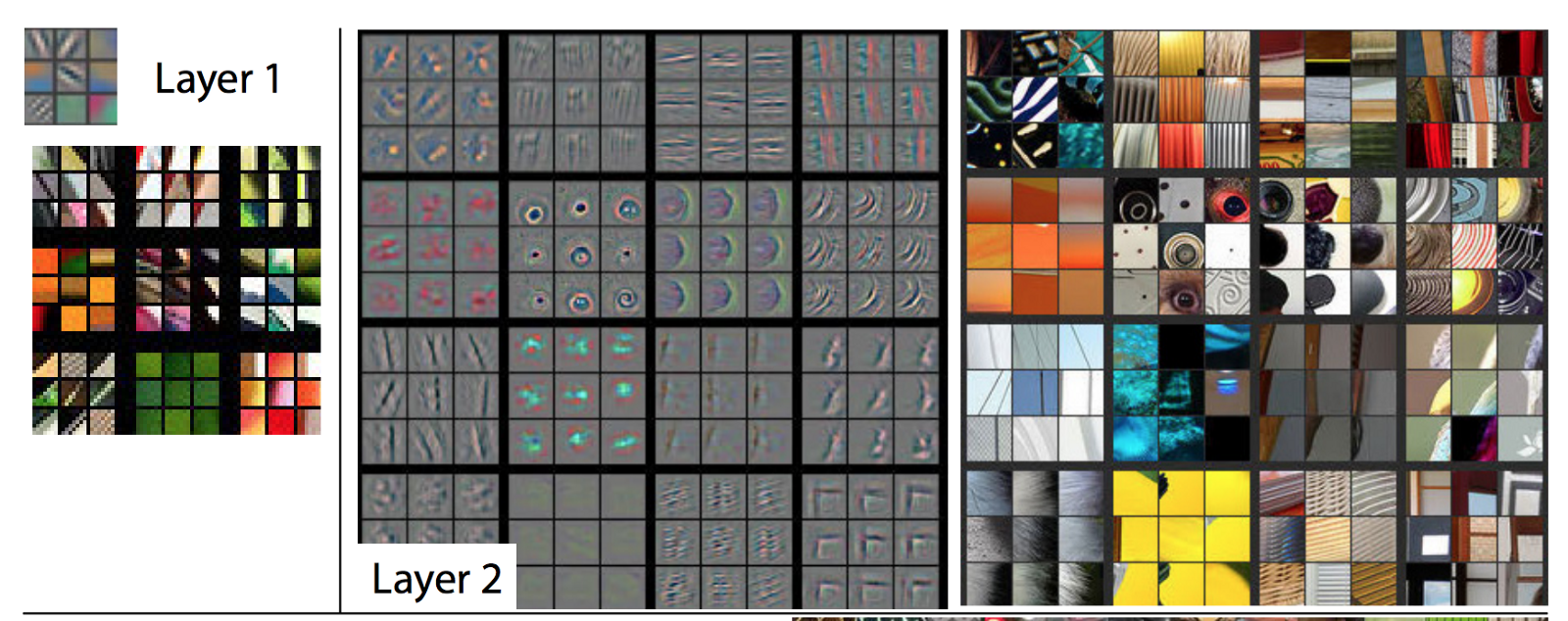
The first lesson focuses on image classification via transfer learning. They provide a pre-trained ResNet-34 network that has learned weights using the ImageNet dataset. This has allowed it to learn various things about the natural world such as the existence of edges, corners, patterns and text.
After creating a competent pet classifier they recommend that students go out and try to use the same approach on a dataset of their own creation. For my part I’ve decided to try their approach on three different datasets, each chosen to be slightly more challenging than the last:
- Impressionist Paintings vs. Modernist Paintings
- Kittens vs. Cats
- Counting objects
Paintings
Full notebook on GitHub.
Our first step is simply to import everything that we’ll need from the fastai library:
This file contains hidden or bidirectional Unicode text that may be interpreted or compiled differently than what appears below. To review, open the file in an editor that reveals hidden Unicode characters.
Learn more about bidirectional Unicode characters
| from fastai.vision import * | |
| from fastai.metrics import error_rate |
Next we’ll take a look at the data itself. I’ve saved it in data/paintings. We’ll create an ImageDataBunch which automatically knows how to read labels for our data based off the folder structure. It also automatically creates a validation set for us.
This file contains hidden or bidirectional Unicode text that may be interpreted or compiled differently than what appears below. To review, open the file in an editor that reveals hidden Unicode characters.
Learn more about bidirectional Unicode characters
| path = 'data/paintings/' | |
| data = ImageDataBunch.from_folder(path, train=".", valid_pct=0.2, | |
| ds_tfms=get_transforms(), size=224, num_workers=4).normalize(imagenet_stats) | |
| data.show_batch(rows=3, figsize=(7,8)) |
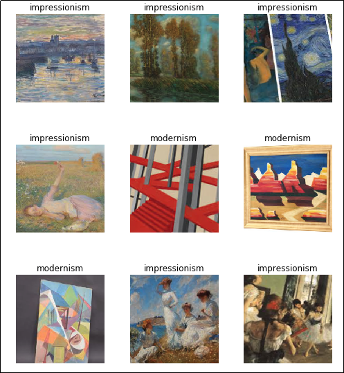
Looking at the above images, it’s fairly easy to differentiate the solid lines of modernism from the soft edges and brush strokes of impressionist paintings. My hope is that this task will be just as easy for a pre-trained neural network that can already recognize edges and identify repeated patterns.
Now that we’ve prepped our dataset, we’ll prepare a learner and let it train for five epochs to get a sense of how well it does.
This file contains hidden or bidirectional Unicode text that may be interpreted or compiled differently than what appears below. To review, open the file in an editor that reveals hidden Unicode characters.
Learn more about bidirectional Unicode characters
| learner = create_cnn(data, models.resnet34, metrics=error_rate) | |
| learner.fit_one_cycle(5) |
| epoch | train_loss | valid_loss | error_rate |
|---|---|---|---|
| 1 | 0.976094 | 0.502022 | 0.225000 |
| 2 | 0.683104 | 0.202733 | 0.100000 |
| 3 | 0.488111 | 0.158647 | 0.100000 |
| 4 | 0.383773 | 0.142937 | 0.050000 |
| 5 | 0.321568 | 0.141001 | 0.050000 |
Looking good! With virtually no effort at all we have a classifier that reaches 95% accuracy. This task proved to be just as easy as expected. In the notebook we take things a further by choosing better learning rate and training for a little while longer before ultimately getting 100% accuracy.
Cats vs. Kittens
Full notebook on GitHub.
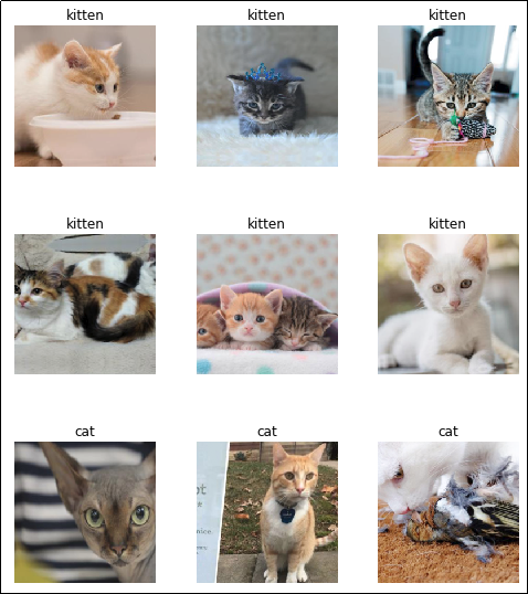
The painting task ended up being as easy as we expected. For our second challenge we’re going to look at a dataset of about 180 cats and 180 kittens. Cats and kittens share many features (fur, whiskers, ears etc.) which seems like it would make this task harder. That said, a human can look at pictures of cats and kittens and easily differentiate between them.
This time our data is located in data/kittencat so we’ll go ahead and load it up.
This file contains hidden or bidirectional Unicode text that may be interpreted or compiled differently than what appears below. To review, open the file in an editor that reveals hidden Unicode characters.
Learn more about bidirectional Unicode characters
| from fastai.vision import * | |
| from fastai.metrics import error_rate | |
| path = 'data/kittencat/' | |
| data = ImageDataBunch.from_folder(path, train=".", valid_pct=0.2, | |
| ds_tfms=get_transforms(), size=224, num_workers=4).normalize(imagenet_stats) |
Once again, let’s try a standard fastai CNN learner and run it for about 5 epochs to get a sense for how it’s doing.
This file contains hidden or bidirectional Unicode text that may be interpreted or compiled differently than what appears below. To review, open the file in an editor that reveals hidden Unicode characters.
Learn more about bidirectional Unicode characters
| learner = create_cnn(data, models.resnet34, metrics=error_rate) | |
| learner.fit_one_cycle(5) |
| epoch | train_loss | valid_loss | error_rate |
|---|---|---|---|
| 1 | 0.887721 | 0.633843 | 0.378788 |
| 2 | 0.732651 | 0.336768 | 0.136364 |
| 3 | 0.569540 | 0.282584 | 0.136364 |
| 4 | 0.492754 | 0.278653 | 0.151515 |
| 5 | 0.425181 | 0.280318 | 0.136364 |
So we’re looking at about 86% accuracy. Not quite the 95% we saw when classifying paintings but perhaps we can push it a little higher by choosing a good learning rate and running our model for longer.
Below we are going to use the “Learning Rate Finder” to (surprise, surprise) find a good learning rate. We’re looking for portions of the plot in which the graph steadily decreased.
This file contains hidden or bidirectional Unicode text that may be interpreted or compiled differently than what appears below. To review, open the file in an editor that reveals hidden Unicode characters.
Learn more about bidirectional Unicode characters
| learner.save('stage-1') | |
| learner.unfreeze() | |
| learner.lr_find() | |
| learner.recorder.plot() |
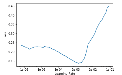
It looks like there is a sweetspot between 1e-5 and 1e-3. We’ll shoot for the ‘middle’ and just use 1e-4. We’ll also run for 15 epochs this time to allow more time for learning.
This file contains hidden or bidirectional Unicode text that may be interpreted or compiled differently than what appears below. To review, open the file in an editor that reveals hidden Unicode characters.
Learn more about bidirectional Unicode characters
| learner.fit_one_cycle(15, max_lr=slice(1e-4)) |
| epoch | train_loss | valid_loss | error_rate |
|---|---|---|---|
| 1 | 0.216681 | 0.285061 | 0.121212 |
| 2 | 0.228469 | 0.287646 | 0.121212 |
| … | … | … | … |
| 14 | 0.148541 | 0.216946 | 0.075758 |
| 15 | 0.141137 | 0.215242 | 0.075758 |
Not bad! With a little bit of learning rate tuning, we were able to get a validation accuracy of about 92% which is much better than I expected considering we had less than 200 examples of each class. I imagine if we collected a larger dataset we could do even better.
Counting Objects
Full notebook on GitHub.
For my last task I wanted to see whether or not we could train a ResNet to “count” identical objects. So far we have seen that these networks excel at distinguishing between different objects, but can these networks also identify multiple occurrences of something?
Note: I specifically chose this task because I don’t believe it should be possible for a vanilla ResNet to accomplish this task. A typical convolutional network is set up to differentiate between classes based on the features of those classes, but there is nothing in a convolutional network that suggests to me that it should be able to count objects with identical features.
For this challenge we are going to synthesize our own dataset using matplotlib. We’ll simply generate plots with the correct number of circles in them as shown below:
This file contains hidden or bidirectional Unicode text that may be interpreted or compiled differently than what appears below. To review, open the file in an editor that reveals hidden Unicode characters.
Learn more about bidirectional Unicode characters
| import random | |
| import numpy as np | |
| import matplotlib.pyplot as plt | |
| def createNonOverlappingPoints(numElements): | |
| x = np.zeros((numElements)) + 2 #Place the cirlces offscreen | |
| y = np.zeros((numElements)) + 2 #Place the circles offscreen | |
| for i in range(0, numElements): | |
| foundNewCircle = False | |
| #Loop until we find a non-overlapping position for our new circle | |
| while not foundNewCircle: | |
| randX = random.uniform(-1, 1) | |
| randY = random.uniform(-1, 1) | |
| distanceFromOtherCircles = np.sqrt(np.square(x – randX) + np.square(y – randY)) | |
| # Ensure that this circle is far enough away from all others | |
| if np.all(distanceFromOtherCircles > 0.2): | |
| break | |
| x[i] = randX | |
| y[i] = randY | |
| return x, y | |
| x, y = createNonOverlappingPoints(10) | |
| plt.scatter(x,y, s=200) | |
| plt.axes().set_aspect('equal', 'datalim') # before `plt.show()` | |
| plt.show() |
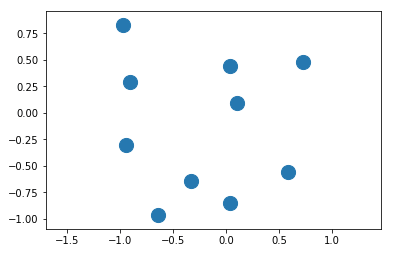
There are some things to note here:
- When we create a dataset like this, we’re in uncharted territory as far as the pre-trained weights are concerned. Our network was trained on photographs of the natural world and expects its inputs to come from this distribution. We’re providing inputs from a completely different distribution (not necessarily a harder one!) so I wouldn’t expect transfer learning to work as flawlessly as it did in previous examples.
- Our dataset might be trivially easy to learn. For example, if we wrote an algorithm that simply counted the number of “blue” pixels we could very accurately figure out how many circles were present as all circles are the same size.
We don’t need to hypothesize any further, though. We can just create our ImageDataBunch and pass it to a learner to see how well it does. For now we’ll just use a dataset with 1-5 elements.
This file contains hidden or bidirectional Unicode text that may be interpreted or compiled differently than what appears below. To review, open the file in an editor that reveals hidden Unicode characters.
Learn more about bidirectional Unicode characters
| path = 'data/counting' | |
| data = ImageDataBunch.from_folder(path, train=".", valid_pct=0.2, | |
| ds_tfms=get_transforms(), size=224, num_workers=4).normalize(imagenet_stats) | |
| data.show_batch(rows=3, figsize=(7,8)) |
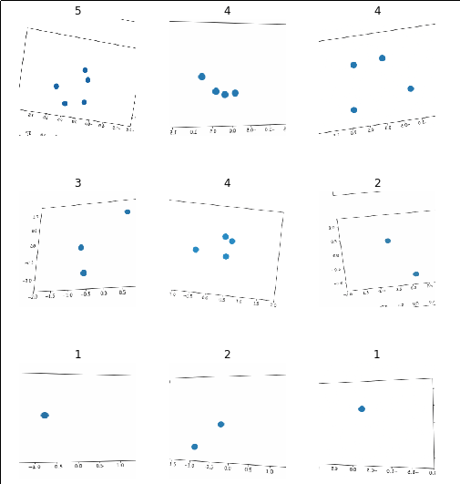
Let’s create our learner and see how well it does with the defaults after 3 epochs.
This file contains hidden or bidirectional Unicode text that may be interpreted or compiled differently than what appears below. To review, open the file in an editor that reveals hidden Unicode characters.
Learn more about bidirectional Unicode characters
| learner = create_cnn(data, models.resnet34, metrics=error_rate) | |
| learner.fit_one_cycle(3) |
| epoch | train_loss | valid_loss | error_rate |
|---|---|---|---|
| 1 | 1.350247 | 0.767537 | 0.346000 |
| 2 | 0.930266 | 0.469457 | 0.165000 |
| 3 | 0.739811 | 0.415282 | 0.136000 |
So without any changes we’re sitting at over 85% accuracy. This surprised me as I thought this task would be harder for our neural network as each object it was counting has identical features. If we run this experiment again with a learning rate of 1e-4 and for 15 cycles things get even better:
| epoch | train_loss | valid_loss | error_rate |
|---|---|---|---|
| 1 | 0.657094 | 0.406908 | 0.133000 |
| 2 | 0.632255 | 0.337327 | 0.100000 |
| … | … | … | … |
| 14 | 0.236516 | 0.039613 | 0.002000 |
| 15 | 0.264761 | 0.037968 | 0.002000 |
Wow! We’ve pushed the accuracy up to 99%!
Ugh. This seems wrong to me…
I am not a deep learning pro but every fiber of my being screams out against convolutional networks being THIS GOOD at this task. I specifically chose this task to try to find a failure case! My understanding is that they should be able to identify composite features that occur in an image but there is nothing in there that says they should be able to count (or have any notion of what counting means!)
What I would guess is happening here is that there are certain visual patterns that can only occur for a given number of circles (for example, one circle can never create a line) and that our network uses these features to uniquely identify each class. I’m not sure how to prove this but I have an idea of how we might break it. Maybe we can put so many circles on the screen that the unique patterns will become very hard to find. For example, instead of trying 1-5 circles, let’s try counting images that have 45-50 circles.
After re-generating our data (see Notebook for details) we can visualize it below:
This file contains hidden or bidirectional Unicode text that may be interpreted or compiled differently than what appears below. To review, open the file in an editor that reveals hidden Unicode characters.
Learn more about bidirectional Unicode characters
| path = 'data/counting' | |
| np.random.seed(42) | |
| data = ImageDataBunch.from_folder(path, train=".", valid_pct=0.2, | |
| ds_tfms=get_transforms(), size=224, num_workers=4).normalize(imagenet_stats) | |
| data.show_batch(rows=3, figsize=(7,8)) |
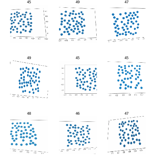
Now we can run our learner against this and see how it does:
This file contains hidden or bidirectional Unicode text that may be interpreted or compiled differently than what appears below. To review, open the file in an editor that reveals hidden Unicode characters.
Learn more about bidirectional Unicode characters
| learner = create_cnn(data, models.resnet34, metrics=error_rate) | |
| learner.fit_one_cycle(3) |
| epoch | train_loss | valid_loss | error_rate |
|---|---|---|---|
| 1 | 2.132017 | 2.023042 | 0.795833 |
| 2 | 1.861990 | 1.643421 | 0.711667 |
| 3 | 1.749233 | 1.663559 | 0.748333 |
This file contains hidden or bidirectional Unicode text that may be interpreted or compiled differently than what appears below. To review, open the file in an editor that reveals hidden Unicode characters.
Learn more about bidirectional Unicode characters
| learner = create_cnn(data, models.resnet34, metrics=error_rate) | |
| learner.fit_one_cycle(3) |
Hah! That’s more like it. Now our network can only achieve ~25% accuracy which is slightly better than chance (1 in 5). Playing around with learning rate I was only able to achieve 27% on this task.
This makes more sense to me. There are no “features” in this image that would allow a network to look at it and instantly know how many circles are present. I suspect most humans can also not glance at one of these images and know whether or not there are 45 or 46 elements present. I suspect we would have to fall back to a different approach and manually count them out.
Update
It turns out that we CAN make this work! We just have to use more sensible transformations. For more info see my next post: Image Classification: Counting Part II.
