Part of the series Learn TensorFlow Now
In previous posts, we simply passed raw images to our neural network. Other forms of machine learning pre-process input in various ways, so it seems reasonable to look at these approaches and see if they would work when applied to a neural network for image recognition.
Zero Centered Mean
One characteristic we desire from any learning algorithm is for it to generalize across different input distributions. For example, let’s imagine we design an algorithm for predicting whether or not the price of a house is “High” or “Low“. As input it takes:
- Number of Rooms
- Price of House
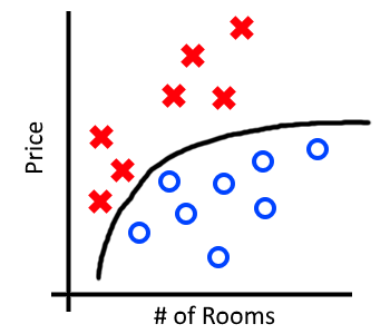
Below is some made-up data for the city of Boston. I’ve marked “High” in red, “Low” in blue and a reasonable decision boundary that our algorithm might learn in black. Our decision boundary correctly classifies all examples of “High” and “Low“.
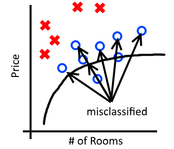
What happens when we take this model and apply it to houses in New York where houses are much more expensive? Below we can see that the model does not generalize and incorrectly classifies many “Low” house prices as “High“.
In order to fix this, we want to take all of our data and zero-center it. To do this, we subtract the mean of each feature from from each data-point. For our examples this would look something like:

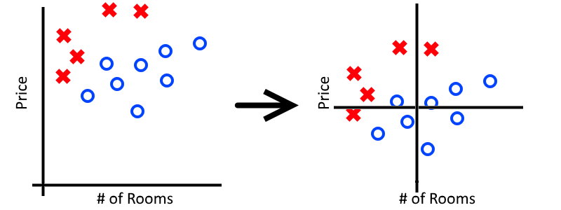
Notice that we zero-center the mean for both the “Price” feature as well as the “Number of Rooms” feature. In general we don’t know which features might cause problems and which ones will not, so it’s easier just to zero-center them all.
Now that our data has a zero-centered mean, we can see how it would be easier to draw a single decision boundary that would accurately classify points from both Boston and New York. Zero centering our mean is one technique for handling data that comes from different distributions.
Changing Distributions in Images
It’s easy to see how the distribution of housing prices changes in different cities, but what would changes in distribution look like when we’re talking about images? Let’s imagine that we’re building an image classifier to distinguish between pictures of cats and pictures of dogs. Below is some sample data:
Training Data
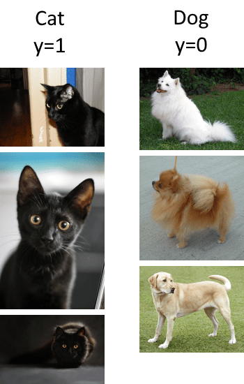
Test Data
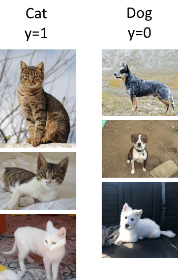
In the above classification task our cat images are coming from different distributions in our training and test sets. Our training set seems to contain exclusively black cats while our test set has a mix of colors. We would expect our classifier to fail on this task unless we take some time to fix our distribution problems. One way to fix this problem would be to fix our training set and ensure it contains many different colors of cats. Another approach we might take would be to zero-center the images, as we did with our housing prices.
Zero Centering Images
Now that we understand zero-centered means, how can we use this to improve our neural network? Recall that each pixel in an image is a feature, analogous to “Price” or “Number of Rooms” in our housing example. Therefore, we have to calculate the mean value for each pixel across the entire dataset. This gives us a 32x32x3 “mean image” which we can then subtract from every image we pass to our neural network.
You mean have noticed that the mean_image was automatically created for us when we called cifar_data_loader.load_data():
This file contains hidden or bidirectional Unicode text that may be interpreted or compiled differently than what appears below. To review, open the file in an editor that reveals hidden Unicode characters.
Learn more about bidirectional Unicode characters
| (train_images, train_labels, test_images, test_labels, mean_image) = cifar_data_loader.load_data() | |
| print(mean_image.shape) #32x32x3 |
The mean image for the CIFAR-10 dataset looks something like:

Now we simply need to subtract the mean image from the input images in our neural network:
This file contains hidden or bidirectional Unicode text that may be interpreted or compiled differently than what appears below. To review, open the file in an editor that reveals hidden Unicode characters.
Learn more about bidirectional Unicode characters
| input_minus_mean = input – mean_image #Subtract mean from input images | |
| layer1_weights = tf.get_variable("layer1_weights", [3, 3, 3, 64], initializer=tf.contrib.layers.variance_scaling_initializer()) | |
| layer1_bias = tf.Variable(tf.zeros([64])) | |
| layer1_conv = tf.nn.conv2d(input_minus_mean, filter=layer1_weights, strides=[1,1,1,1], padding='SAME') #Use input_minus_mean now | |
| layer1_out = tf.nn.relu(layer1_conv + layer1_bias) |
After running our network we’re greeted with the following output:
Cost: 131.964
Accuracy: 11.9999997318 %
Cost: 1.91737
Accuracy: 23.9999994636 %
Cost: 1.7101
Accuracy: 33.0000013113 %

...

Cost: 0.494887
Accuracy: 86.0000014305 %
Cost: 0.47334
Accuracy: 83.9999973774 %
Test Cost: 1.04789093912
Test accuracy: 72.5600001812 %
A test accuracy of 72.5% is a marginal increase over our previous result of 70.9% and it’s possible that our improvement is entirely due to chance. So why doesn’t zero centering the mean help much? Recall that zero-centering the mean leads to the biggest improvements when our data comes from different distributions. In the case of CIFAR-10, we have little reason to suspect that our portions of our images are obviously of different distributions.
Despite seeing only marginal improvements, we’ll continue to subtract the mean image from our input images. It imposes only a very small performance penalty and safeguards us against problems with distributions we might not anticipate in future datasets.
