Full Notebook on GitHub.
Usually when we work with a neural network we treat it as a black box. We can pull a few knobs and levers (learning rate, weight decay, etc.) but for the most part we’re stuck looking at the inputs and outputs to the network. For most of us this means we simply plot loss and maybe a target metric like accuracy as training progresses.
This state of affairs will leave almost anyone from a software background feeling a little empty. After all, we’re used to writing code in which we try to understand every bit of internal state. And if something goes wrong, we can always use a debugger to step inside and see exactly what’s going on. While we’re never going to get to that point with neural networks, it feels like we should at least be able to take a step in that direction.
To that end, let’s try taking a look at the internal activations of our neural network. Recall that a neural network is divided up into many layers, each with intermediate output activations. Our goal will be to simply visualize those activations as training progresses. For this we’ll use fastai’s HookCallback, but since fastai abstracts over PyTorch, the same general approach would work for PyTorch as well.
First we’ll start by defining a StoreHook class that initializes itself at the beginning of training and keeps track of output activations after each batch. However, instead of saving each output activation (there can be tens of thousands) let’s use .histc() to count the number of activations across 40 different ranges (or buckets). This allows us to determine whether most activations are high or low without having to keep them all around.
This file contains hidden or bidirectional Unicode text that may be interpreted or compiled differently than what appears below. To review, open the file in an editor that reveals hidden Unicode characters.
Learn more about bidirectional Unicode characters
| # Modified from: https://forums.fast.ai/t/confused-by-output-of-hook-output/29514/4 | |
| class StoreHook(HookCallback): | |
| def on_train_begin(self, **kwargs): | |
| super().on_train_begin(**kwargs) | |
| self.hists = [] | |
| def hook(self, m, i, o): | |
| return o | |
| def on_batch_end(self, train, **kwargs): | |
| if (train): | |
| self.hists.append(self.hooks.stored[0].cpu().histc(40,0,10)) |
Next we’ll define a method that simply creates a StoreHook for a given module in our neural network. We attach our StoreHook as a callback for our fastai cnn_learner.
This file contains hidden or bidirectional Unicode text that may be interpreted or compiled differently than what appears below. To review, open the file in an editor that reveals hidden Unicode characters.
Learn more about bidirectional Unicode characters
| # Simply pass in a learner and the module you would like to instrument | |
| def probeModule(learn, module): | |
| hook = StoreHook(learn, modules=flatten_model(module)) | |
| learn.callbacks += [ hook ] | |
| return hook |
And that’s pretty much it. Despite not being much code, we’ve got everything we need to monitor the activations of any module on any learner.
Let’s see those activations!
To keep things simple we’ll use ResNet-18, a relatively small version of the network. It looks something like:

We’ll instrument conv1, conv2_x, conv3_x, conv4_x, and conv5_x.
When we run ResNet-18 against MNIST for three epochs, we get an error rate of approximately 3.4% (ie. 96.6% accuracy) and we can plot our activations:
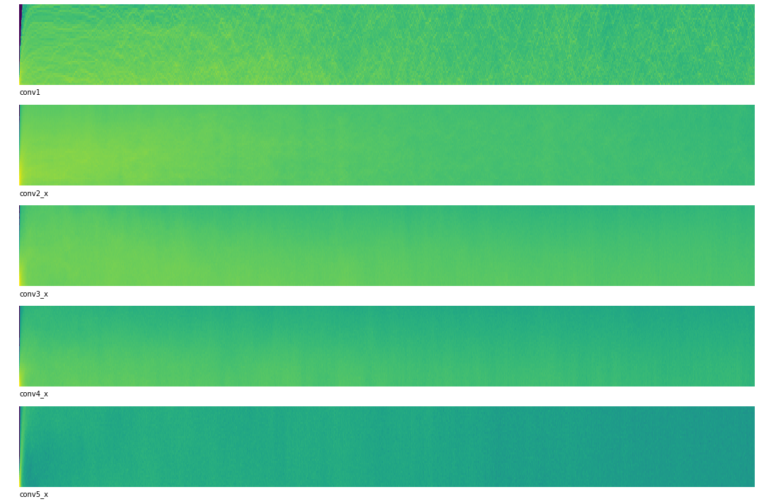
In the above:
- The x-axis represents time (or batch number)
- The y-axis represents the magnitude of activations.
- More yellow indicates more activations at that magnitude
- More blue indicates fewer activations at that magnitude.
If you look very closely at the beginning, most activations start out near zero and as training progresses they quickly become more evenly distributed. This is probably a good thing and our low error rate confirms this.
So if this is what “good” learning looks like, what does “bad” learning look like?
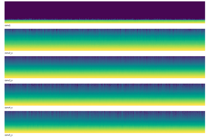
Let’s crank up our learning rate to from 1e-2 to 1 and re-run. This time we get an error rate of 89.9% (ie. accuracy of 10.1%) and activations that look like: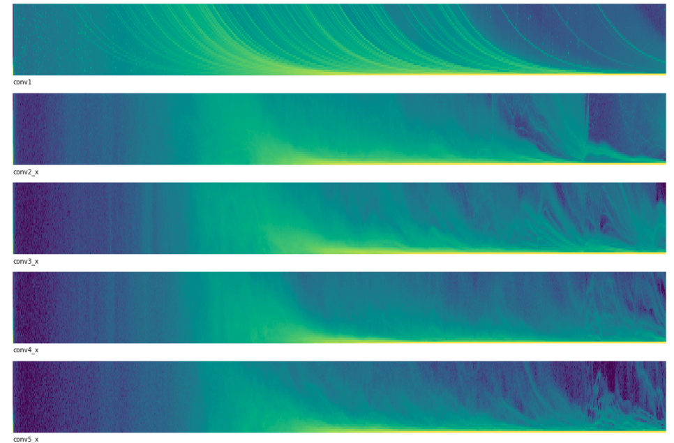
This time as we move through time we see that our activations trend downward toward zero. This is probably bad. If most of our activations are zero then the gradients for these units will also be zero and the network will never be able to update these bad units.
Show me something useful
The above example was a little contrived. Will plotting these activations ever actually be useful?
Recently I’ve been working on Kaggle’s Freesound Audio Tagging challenge in which contestants try to determine what sounds are present in a given audio clip. By converting all the sounds into spectrograms we can rephrase this problem as an image recognition problem and use ResNet-18 against it.
I ran my first network against the data with:
This file contains hidden or bidirectional Unicode text that may be interpreted or compiled differently than what appears below. To review, open the file in an editor that reveals hidden Unicode characters.
Learn more about bidirectional Unicode characters
| learn = cnn_learner(data, models.resnet18, pretrained=False, metrics=[f_score]) | |
| learn.unfreeze() | |
| learn.fit_one_cycle(10, max_lr=slice(1e-6,1e-2)) |
And visualized the activations with:
This seems even weirder than before. None of our layers have evenly distributed distributions of activations and the first layer looks completely broken. Almost all of the first layer’s activations are near zero!
After reflecting on this problem I realized that the problem was I was using discriminitive learning rates. That is, I train the early layers with a very small learning rate of 1e-6 and the latter layers with a larger rate of 1e-2. This approach is very useful when training a network that had been pretrained on another dataset such as ImagetNet. However in this particular competition we weren’t allowed to use a pretrained model! In essence this meant that after randomly initializing the first few layers, they weren’t able to learn anything because the learning rate was so small.
The fix was to use a single learning rate for all layers:
This file contains hidden or bidirectional Unicode text that may be interpreted or compiled differently than what appears below. To review, open the file in an editor that reveals hidden Unicode characters.
Learn more about bidirectional Unicode characters
| learn.fit_one_cycle(10, max_lr=(1e-2)) |
After this change the activations looked like:
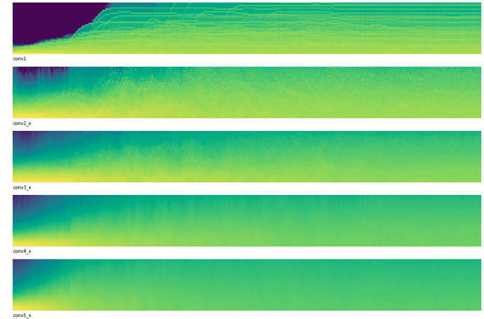
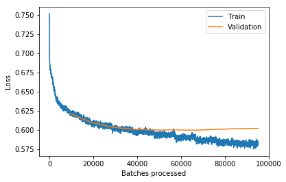
Much better! Our activations started off near zero but we can clearly see that they change as learning progresses. Even our latter layers seem to distribute their activations in a much more balanced way.
Not only do our activations look better, but our network’s score improved as well. This single change improved the f_score of my model from 0.238104 to 0.468753 with a corresponding improvement in loss.
After making this single change: